Multi-Panel Figures in R
Presenting multiple graphs in one figure can be a valuable tool for visualizing data. For example, you might want to compare or contrast different graphs or perhaps emphasize a group of graphs for a report or presentation. There are many methods that we can use to present multiple graphs together in R. This post outlines some possible methods that you can use to present multiple graphs and the potential benefits/drawbacks of each.
Table of Contents
Load in dataset
In all these examples, we will use the penguins dataset in the palmerpenguins package. Instructions to download this package can be found here. Before creating figures from these data, we omitted any rows where values in one or more cells was missing, using the na.omit() function. Additionally, themes are tools that can be used create different aesthetics for figures. In these example figures, we will be using theme_clean() from the ggthemes package to standardize the aesthetics in these figures.
library(palmerpenguins)

?penguins #can be used to find more information about the penguins dataset

data("penguins")
head(penguins)
penguins <- na.omit(penguins)
Using baseR
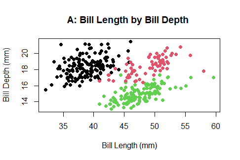
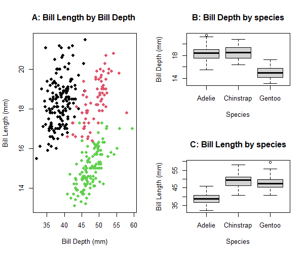
baseR allows you to create a matrix of a plot in one space. However, this matrix can only support plots created using baseR frameworks, so its functionality is limited. Say you are looking at the relationship between bill length and bill depth in penguins. In addition to this relationship, you also want to list information about the distribution of these two variables you are investigating. Individually, each baseR graph will look like this:
plot(penguins$bill_length_mm, penguins$bill_depth_mm,
col= penguins$species,
pch=16,
xlab="Bill Length (mm)", #label for x-axis
ylab="Bill Depth (mm)", #label for y-axis
main="A: Bill Length by Bill Depth ") #plot title
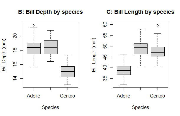
a<- boxplot(penguins$bill_depth_mm ~ penguins$species,
xlab="Species",
ylab="Bill Depth (mm)",
main="B: Bill Depth by species")
b<- boxplot(penguins$bill_length_mm ~ penguins$species,
xlab="Species",
ylab="Bill Length (mm)",
main="C: Bill Length by species")
box <- rbind(a,b)
Tp fit multiple plots on the sample panel, there are a few ways to do this using baseR. Using the par(mfrow=) parameter or layout() functions, we can adjust the plotting space to fit multiple plots.
par() parameter
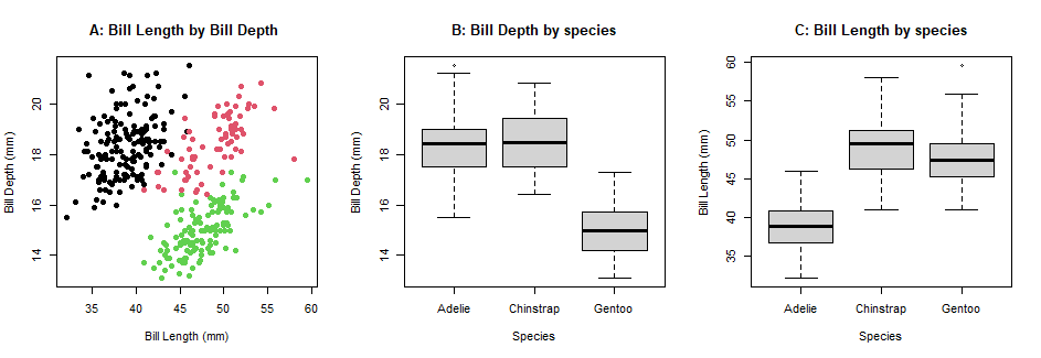
What can the parameter par() do?? par() allows you to adjust plots in the horizontal or vertical plane. However, par() doesn’t allow you to control the proportions of the plotting space, as you can see in the following example:
parameter <- par(mfrow=c(1,3)) #set up the plotting space
parameter <- plot(penguins$bill_length_mm, penguins$bill_depth_mm,
     col= penguins$species,
     pch=16,
     xlab="Bill Length (mm)", #label for x-axis
     ylab="Bill Depth (mm)", #label for y-axis
     main="A: Bill Length by Bill Depth ") #plot title
parameter <- boxplot(penguins$bill_depth_mm ~ penguins$species,
        xlab="Species",
        ylab="Bill Depth (mm)",
        main="B: Bill Depth by species")
parameter <- boxplot(penguins$bill_length_mm ~ penguins$species,
        xlab="Species",
        ylab="Bill Length (mm)",
        main="C: Bill Length by species")
layout() function
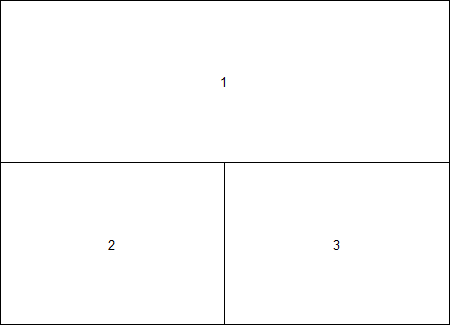
Compared to par() parameter, the layout() function can give you more control over the proportions of the plotting space, for example:
layout(matrix(c(1,1,2,3), 2, 2, byrow = T))
layout.show(n=3)
layout <- layout(matrix(c(1,1,2,3), 2, 2, byrow = F))
layout <- plot(penguins$bill_length_mm, penguins$bill_depth_mm,
     col= penguins$species,
     pch=16,
     xlab="Bill Depth (mm)",
     ylab="Bill Length (mm)",
     main="A: Bill Length by Bill Depth ")
layout <- boxplot(penguins$bill_depth_mm ~ penguins$species,
        xlab="Species",
        ylab="Bill Depth (mm)",
        main="B: Bill Depth by species")
layout <- boxplot(penguins$bill_length_mm ~ penguins$species,
        xlab="Species",
        ylab="Bill Length (mm)",
        main="C: Bill Length by species")
layout <- mtext("Bill Length and Bill Depth by Species", side=3, outer=T, line=-1)
Additional examples of how to use the layout() function can be found here. Using layout() also changes the proportions of the graphs which may affect the final interpretation of results.
The main downside of using par() parameter and layout() function in baseR, is that you can only use plots created using baseR code. While baseR can be useful for creating basic plots, it has limited functionality. The next few sections cover multi-panel figure using plots created with the ggplot2 package, which allows more flexibilty when creating figures.
Load in relevant libraries
library(ggplot2) # to create data visualizations
library(ggthemes) # use themes to clean up the data visualizations
library(Rcolorbrewer) # for multiple color palettes
More information about how to use the RColorBrewer package can be found here. Further information on how to use color to your advantage in ggplots, see here and here.
Create Plots
Now, we are going to create four plots using the ggplot2 package that will be used in the following examples. These four plots will be looking at different relationships of body mass (g) and bill length (mm) separated by species(Adelie, Chinstrap, Gentoo).
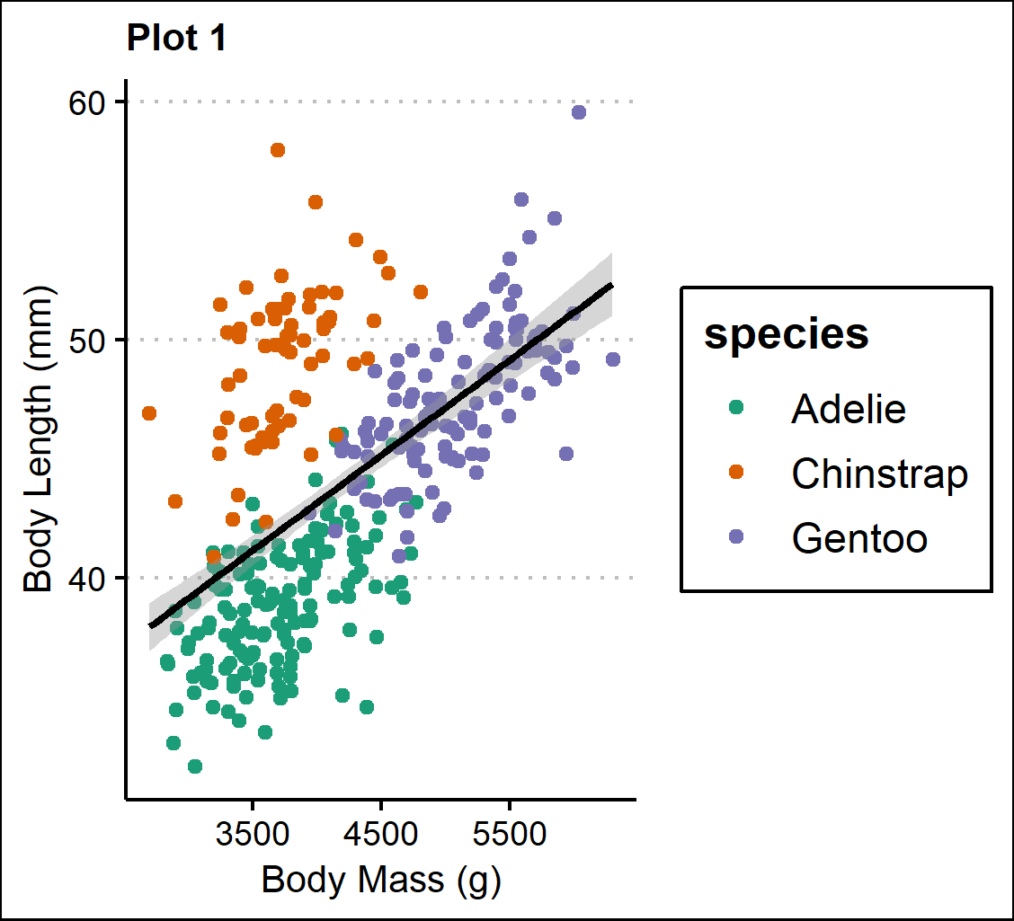
Plot 1 - A scatterplot of body mass (g) and bill length (mm) with a linear regression line. The plots are organized by species.
p1 <- ggplot(penguins,
             aes(x=body_mass_g,y=bill_length_mm,color=species))+
  geom_point(position="jitter")+
  geom_smooth(method=lm , color="black",se=T) +
  scale_color_brewer(palette="Dark2")+
  theme_clean()+
  theme(plot.title=element_text(size=10))+
  labs(title="Plot 1",
       x="Body Mass (g)", y="Body Length (mm)")
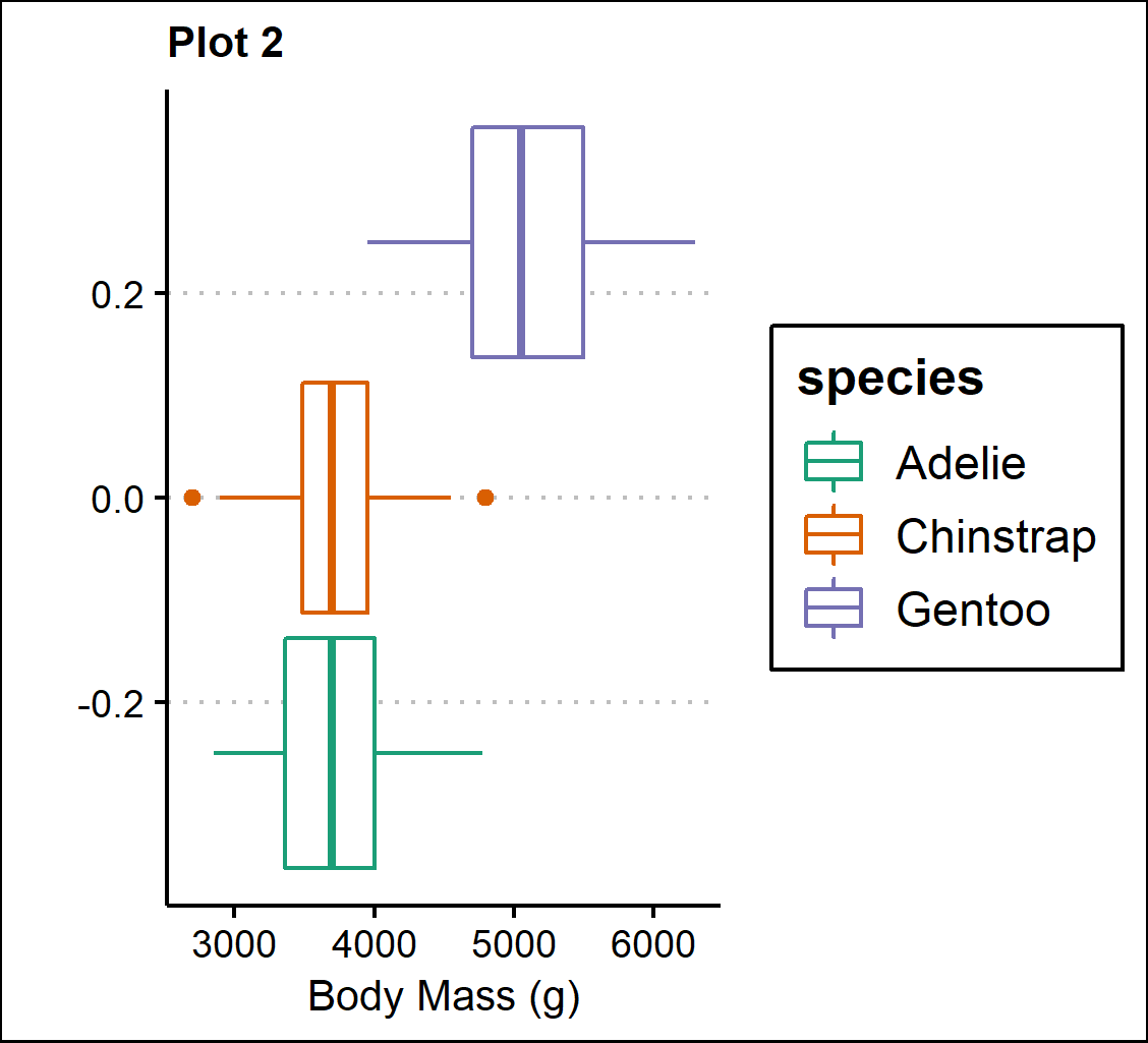
Plot 2 - Boxplots of body mass (g) separated by species.
p2 <- ggplot(penguins, aes(x=body_mass_g, y=n, color=species))+
  geom_boxplot(position="dodge")+
  scale_color_brewer(palette="Dark2")+
  theme_clean()+
  theme(plot.title=element_text(size=10))+
  labs(title="Plot 2",
       x="Body Mass (g)", y="")
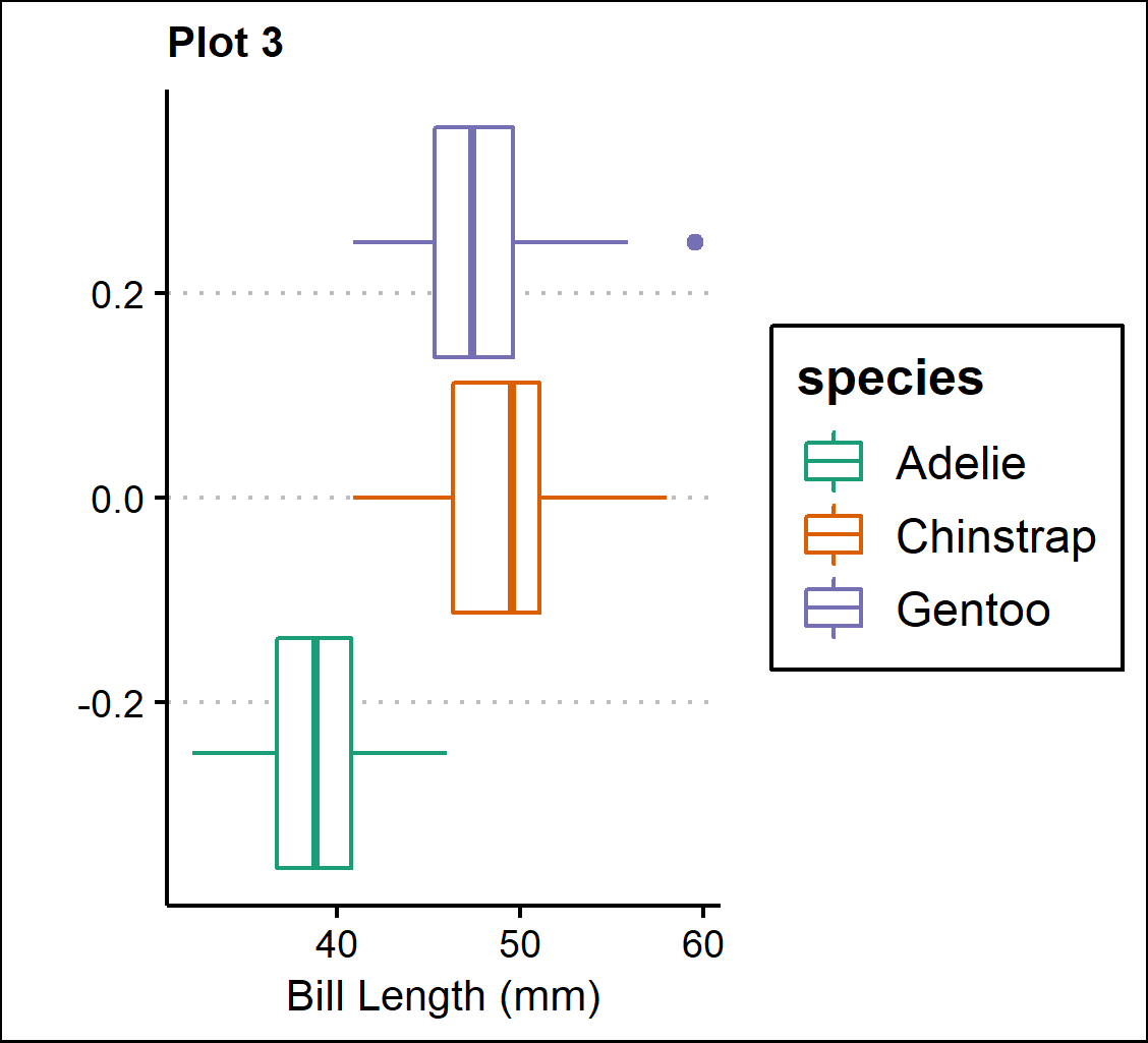
Plot 3 - Boxplots of bill length (mm) separated by species.
p3 <- ggplot(penguins, aes(x=bill_length_mm, y=n, color=species))+
  geom_boxplot(position="dodge")+
  scale_color_brewer(palette="Dark2")+
  theme_clean()+
  theme(plot.title=element_text(size=10))+
  labs(title="Plot 3",
       x="Bill Length (mm)", y="")
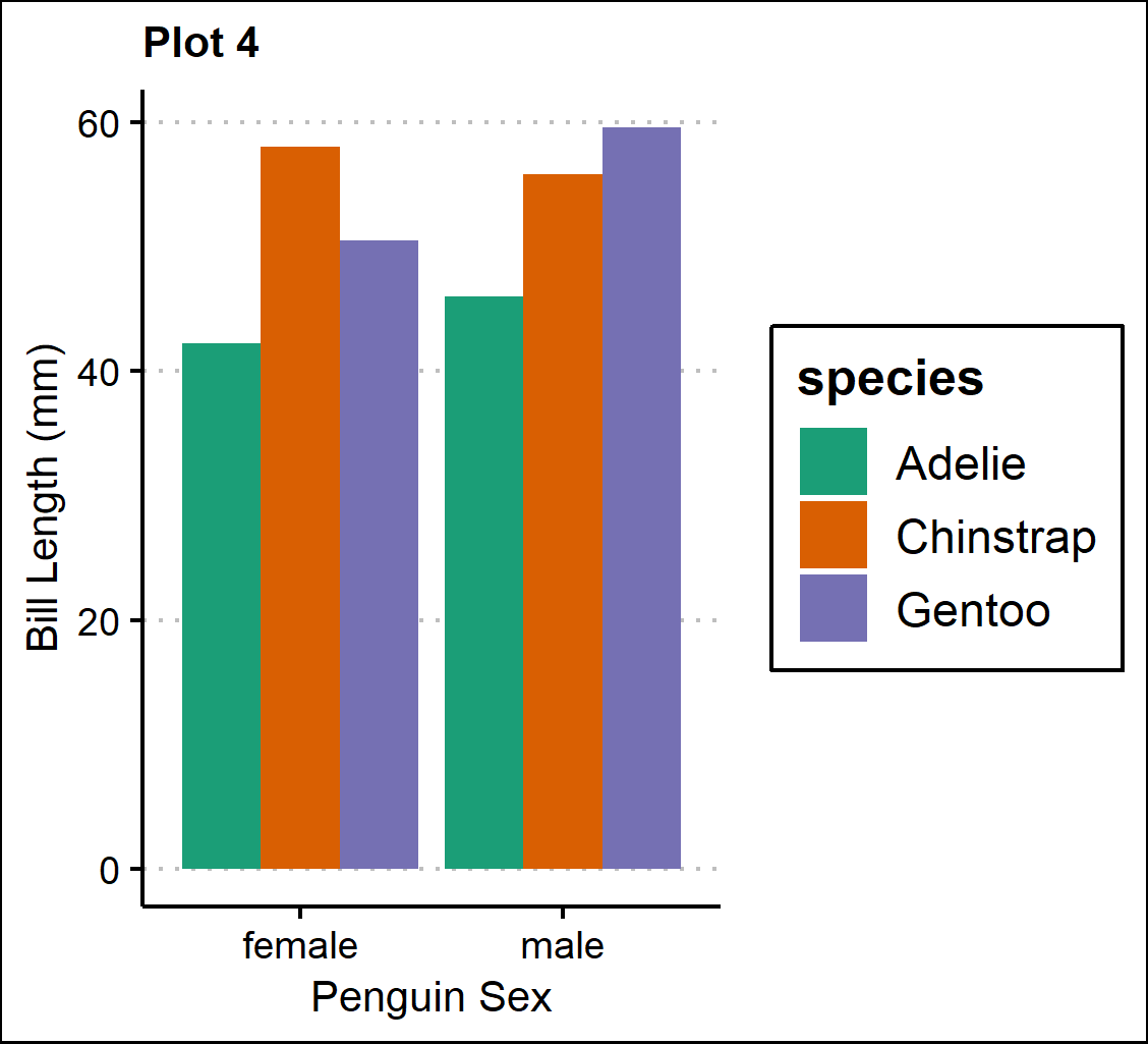
Plot 4 - A barplot of bill length (mm) separated by penguin sex(male & female) on the x-axis and species.
p4 <- ggplot(penguins, aes(x=sex, y=bill_length_mm, fill=species))+
  geom_bar(position="dodge", stat="identity")+
  scale_fill_brewer(palette="Dark2")+
  theme_clean()+
  theme(plot.title=element_text(size=10))+
  labs(title="Plot 4",
       x="Sex", y="Bill Length (mm)")
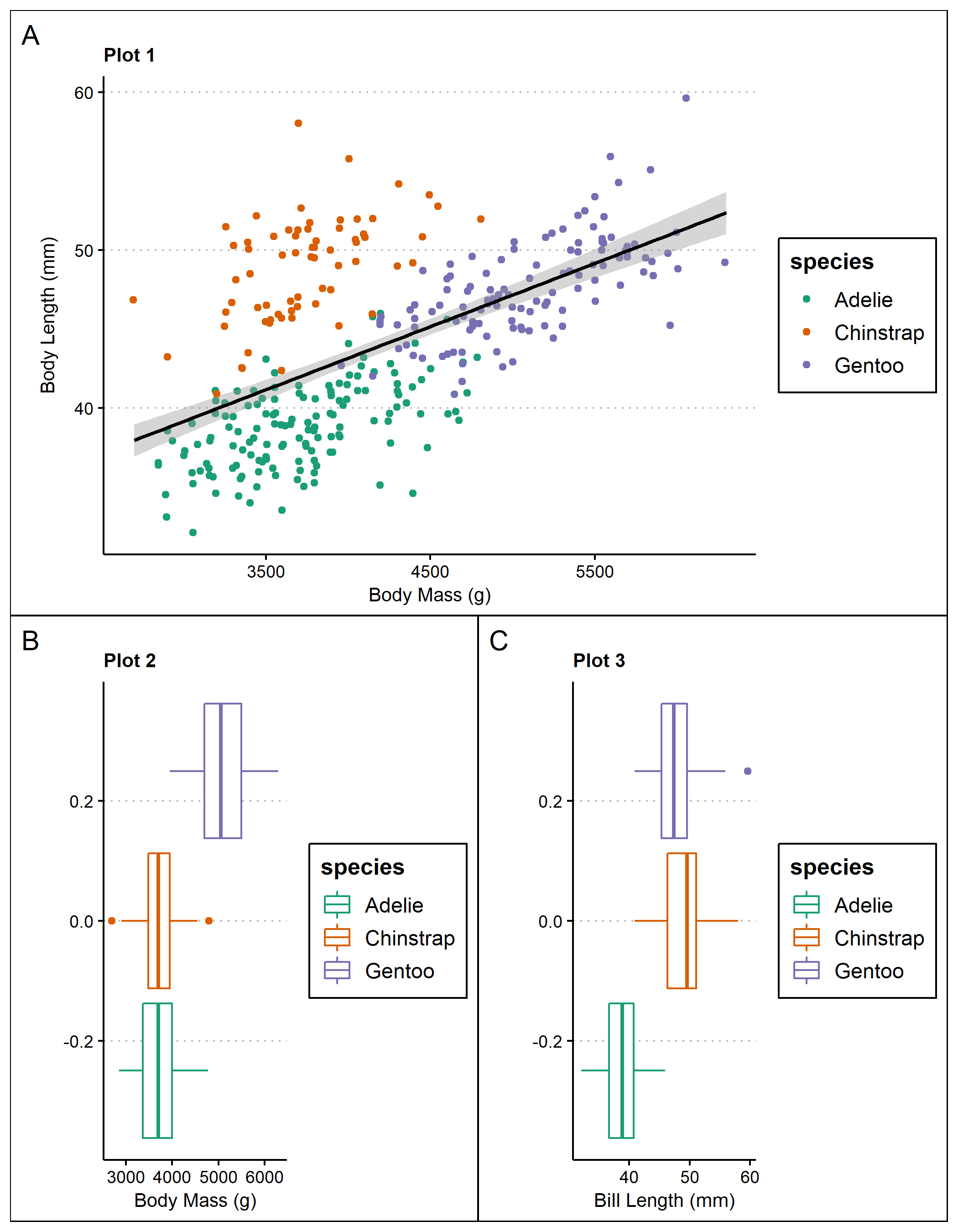
Using patchwork
The patchwork package can be fairly intuitive when it comes to organizing graphs in grids. First, we want to create multi-panel plots, where each plot is next to each other. We can easily adjust the vertical (using “/") and horizontal (using “|") placement of the graphs:
nested <- (p1/(p2|p3))+
  plot_annotation(tag_levels = 'A') #add figure labels
nested #view multi-panel figure
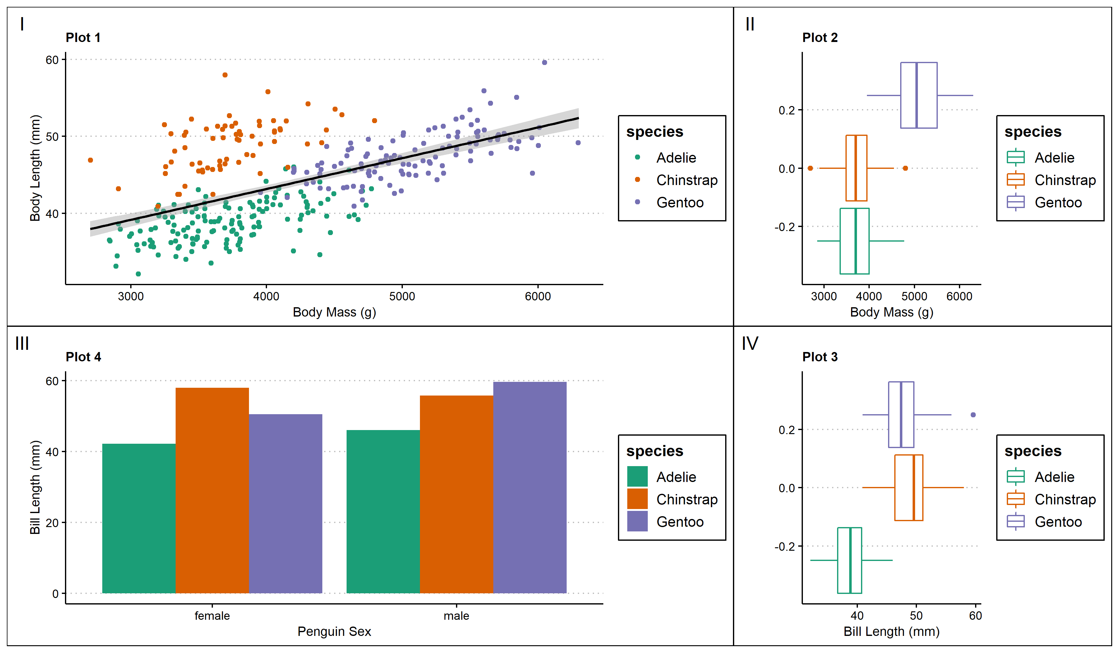
We can also adjust plot placement in the plotting space using the plot_layout() function:
multi <- (p1 + p2 + p4 + p3) +
  plot_layout(widths = c(3,1))+
  plot_annotation(tag_levels = 'I') #add figure labels
multi #view multi-panel figure
Another benefit of using patchwork is that you can add empty spaces within the plotting space.
space <- (p2 + plot_spacer() + p3)/ (plot_spacer() + p4 + plot_spacer())+
  plot_annotation(tag_levels = 'i') #add figure labels
space #view multi-panel figure
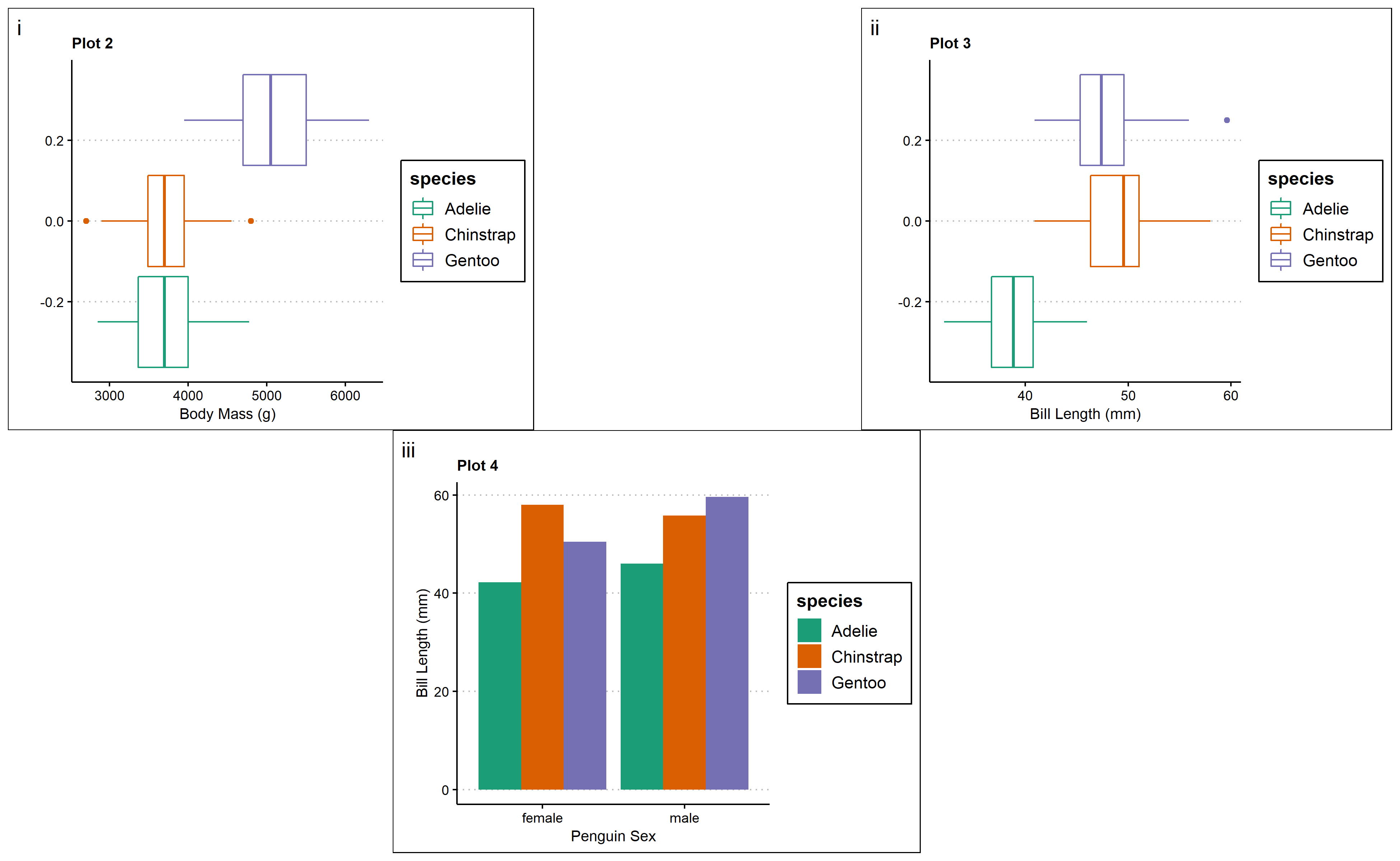
One big downside of using patchwork is that creating common legends in the multi-panel figure is difficult, as you can see in the above images. The legends of each graph are taking up valuable space that could be used for the graph instead.
Using cowplot
patchwork as a package simultaneously aligns and arranges plots at the same time, while the cowplot package can align plots independently of how they are arranged or even put them on top of each other.
For example, cowplot can be used to organize plots into multi-panel grids:
library(cowplot) #load in library to create plot grids
#multi-panel side by side graphs
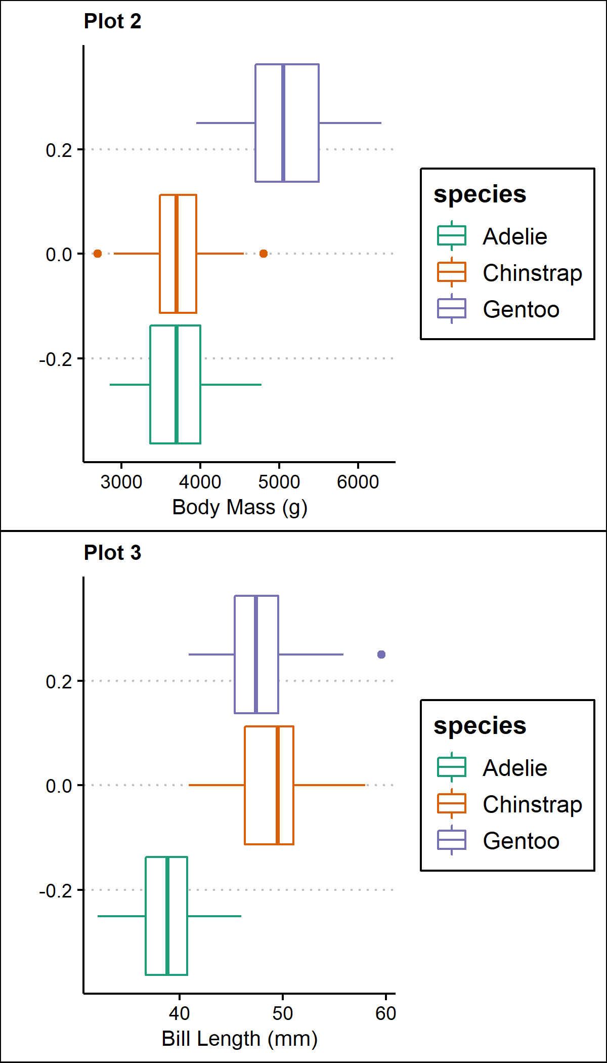
cow <- plot_grid(p2,p3, ncol=1, align = "v", axis="1")
cow #view the multi-panel figure
Additionally, you can remove the y-axis elements from all but the first plot in the bottom row, where two graphs are nested together:
#nested plots
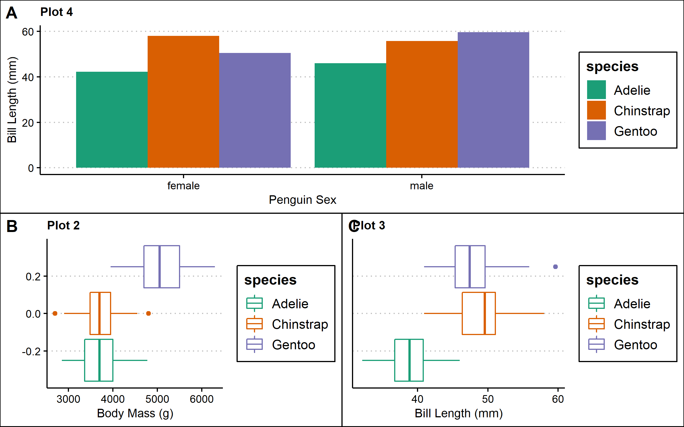
bottom <- plot_grid(p2,p3, labels=c('B','C')) #nest plots at the bottom row
nested <- plot_grid(p4, bottom, labels=c('A',''),ncol=1) #combine plots into one plotting space
nested #view the multi-panel figure
Further, cowplot can be used to arrange plots from different plotting frameworks. For example, you can combine plots made in baseR and ggplot2.
#multiple plotting frameworks
#create a new graph using baseR
p5 <- ~{
par(
mar = c(3, 3, 1, 1),
mgp = c(2, 1, 0)
)
boxplot(penguins$bill_depth_mm ~ penguins$species,
xlab = "Penguin Species", ylab = "Bill Depth (mm)")
}
ggdraw(p5) #save the baseR graph
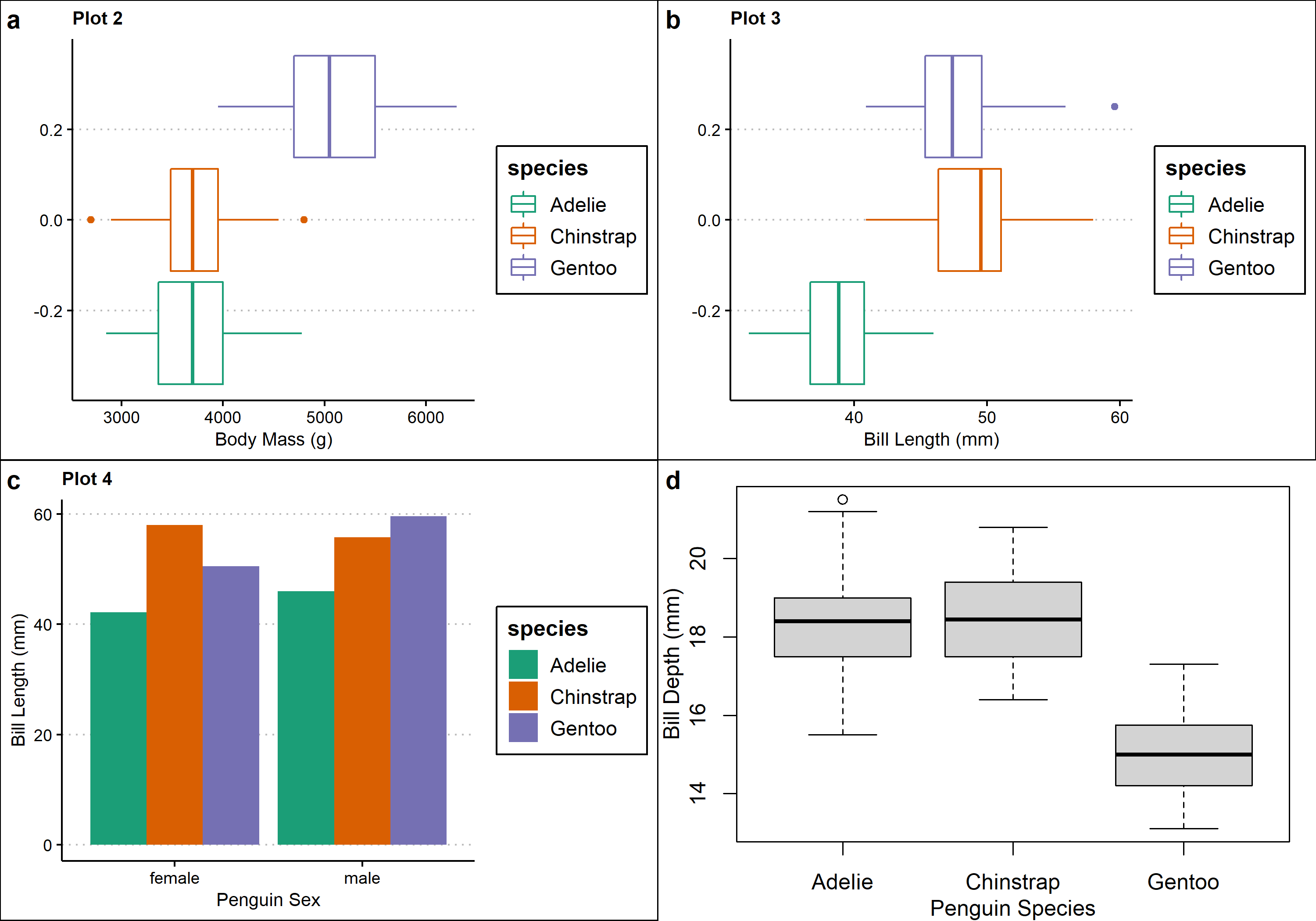
arrange <- plot_grid(p2,p3,p4,p5, labels="auto") #combine the plots into one plotting space
arrange #view the multi-panel figure
As you can see, a major downside to both cowplot and patchwork is that you can’t create a common legend for the multi-panel plot. We can solve this problem using a different method.
Using ggpubr::ggarrange
Using ggpubr::ggarrange provides the most control over the different elements of the plot. You can control the plots, the labels, and easily add a common legend. In contrast, cowplot and patchwork packages do not allow you to create a common legend easily, so a lot of your graph space is taken up by the legend rather than the graph itself.
library(gpubr) #load in library for multi-panel figures
#put all three plots together into one multipanel plot
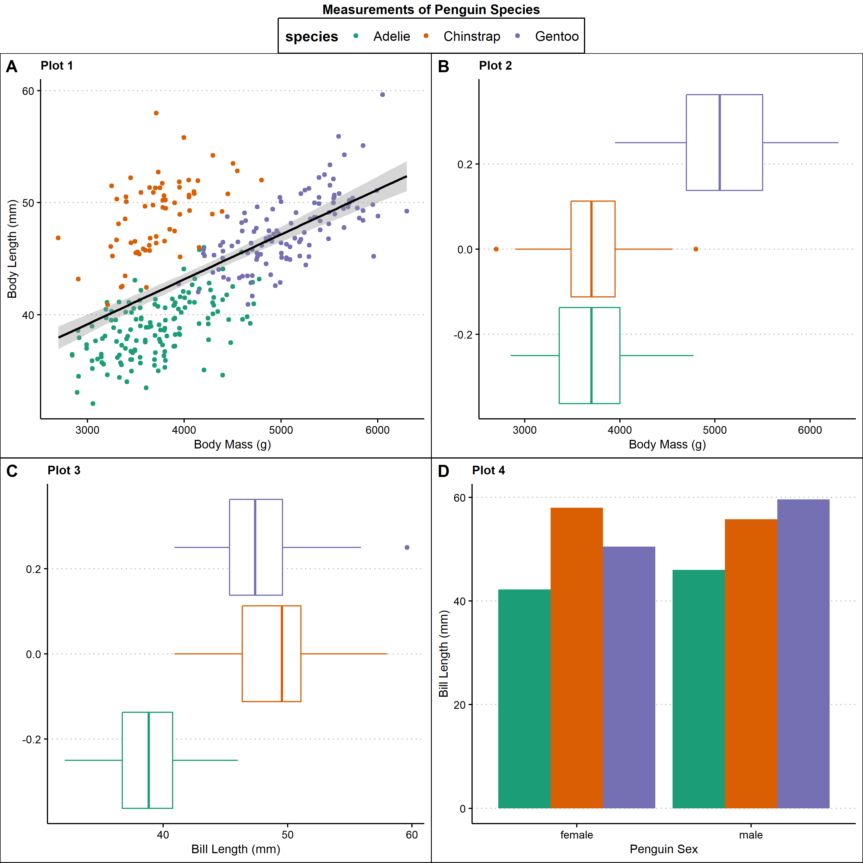
multi_plot<- ggarrange(p1,p2,p3,p4, #plots that are going to be included in this multipanel figure
labels = c("A", "B", "C","D"), #labels given each panel
ncol = 2, nrow = 2, #adjust plot space
common.legend = T) #does the plot have a common legend
#add titles and labels to the multi-panel graph
multi_plot <- annotate_figure(multi_plot,
top = text_grob("Measurements of Penguin Species", color = "black", face = "bold", size = 11))
multi_plot
Specialized multi-panel figures
Marginal Plots
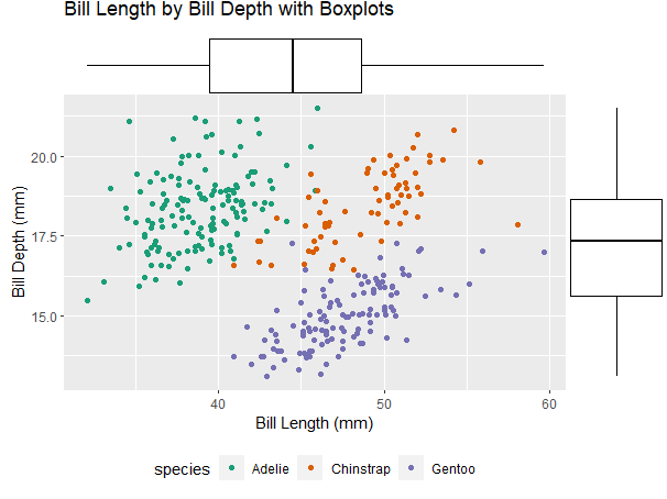
Marginal plots are scatterplots that have histograms or boxplots on the margins of x- and y-axes. This plot helps you examine the relationship and distributions of two variables. Say you want to investigate the relationship between bill length and bill depth and their individual distributions. There are two methods that would allow you to create these plots.
Using baseR
The first method is using the layout() function in baseR. This method requires you to create each plot separately and place them into the plotting matrix, which can get a bit more complicated to organize or process as an R user.
#set plot layout
layout(mat = matrix(c(2, 1, 0, 3),
                    nrow = 2, #number of rows
                    ncol = 2), #number of columns
       heights = c(1, 2),    # Heights of the two rows
       widths = c(2, 1))     # Widths of the two columns
layout.show(3) #see the plot layout
#plot1: scatterplot
par(mar = c(5, 4, 0, 0)) #location of plot
plot(penguins$bill_length_mm,
     penguins$bill_depth_mm,
     xlab = "Bill Length (mm)",
     ylab = "Bill Depth (mm)",
     pch = 16,
     col= penguins$species)
#plot2: top (bill length) boxplot
par(mar = c(0, 4, 0, 0)) #location of plot
boxplot(penguins$bill_length_mm, xaxt = "n",
        yaxt = "n", bty = "n", yaxt = "n",
        col = "white", frame = FALSE, horizontal = TRUE)
#plot3: right (bill depth) boxplot
par(mar = c(5, 0, 0, 0)) #location of plot
boxplot(penguins$bill_depth_mm, xaxt = "n",
        yaxt = "n", bty = "n", yaxt = "n",
        col = "white", frame = F)

using ggExtra::ggMarginal
The second method is using ggExtra::ggMarginal.This method allows you more control over the layers of the figure and is more user friendly.
library(ggplot2) #for creating figures
library(ggExtra) #for building graphs into the margins

marginal <- ggplot(penguins, aes(x=bill_length_mm, y=bill_depth_mm, color=species))+
  geom_point(position="jitter")+
  theme(legend.position = "bottom")+ #change the location of the legend
  labs(title= "Bill Length by Bill Depth with Boxplots", x="Bill Length (mm)", y="Bill Depth (mm)")
marginal<- ggMarginal(marginal, type="boxplot")
marginal #view final plot
ggplot2::facet_wrap
Finally, say you want to create figures to visualize the number of penguins separated by sex and species, two categorical variables. One way of plotting this data is all in one graph:
library(ggplot2) #for creating figures
library(ggthemes) #for figure themes
library(RColorBrewer) #for multiple color palettes
peng <- ggplot(penguins, aes(x=species, fill=sex))+
  geom_bar(position="dodge") +
  scale_fill_brewer(palette="Pastel1")+
  theme_classic()+
  labs(title="Frequency of Species Separated by sex", #change the title of the figure
       x="Species", #change the label of the x axis
       y="Frequency", #change the label of the y axis
       fill="Penguin Sex") #change the title of the legend
peng
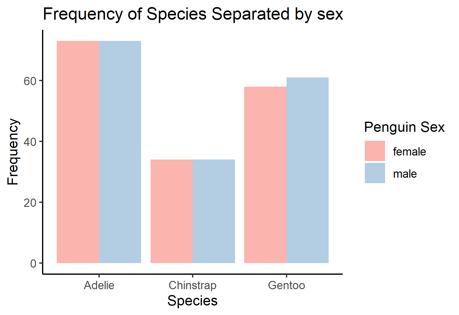
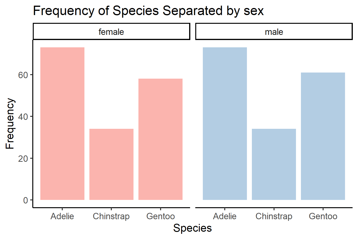
This graph can be a little hard to read. Another method of displaying the count of penguins separated by sex and gender is by using ggplot2:facet_wrap(). These functions will allow you to create multiple panels using information from categorical variables in the data.
This figure might be a bit easier to read because you can more clearly visualize the variables being organized.
peng_facet <- ggplot(penguins, aes(x=species, fill=sex))+
  geom_bar(show.legend = F)+ #remove the legend from the graph
  facet_wrap(~sex) + #create a panel for each sex
  scale_fill_brewer(palette="Pastel1")+ #altering colors of the figure
  theme_classic()+
  labs(title="Frequency of Species Separated by sex", #change the title of the figure
       x="Species", #change the label of the x axis
       y="Frequency", #change the label of the y axis
       fill="Penguin Sex") #change the title of the legend
peng_facet
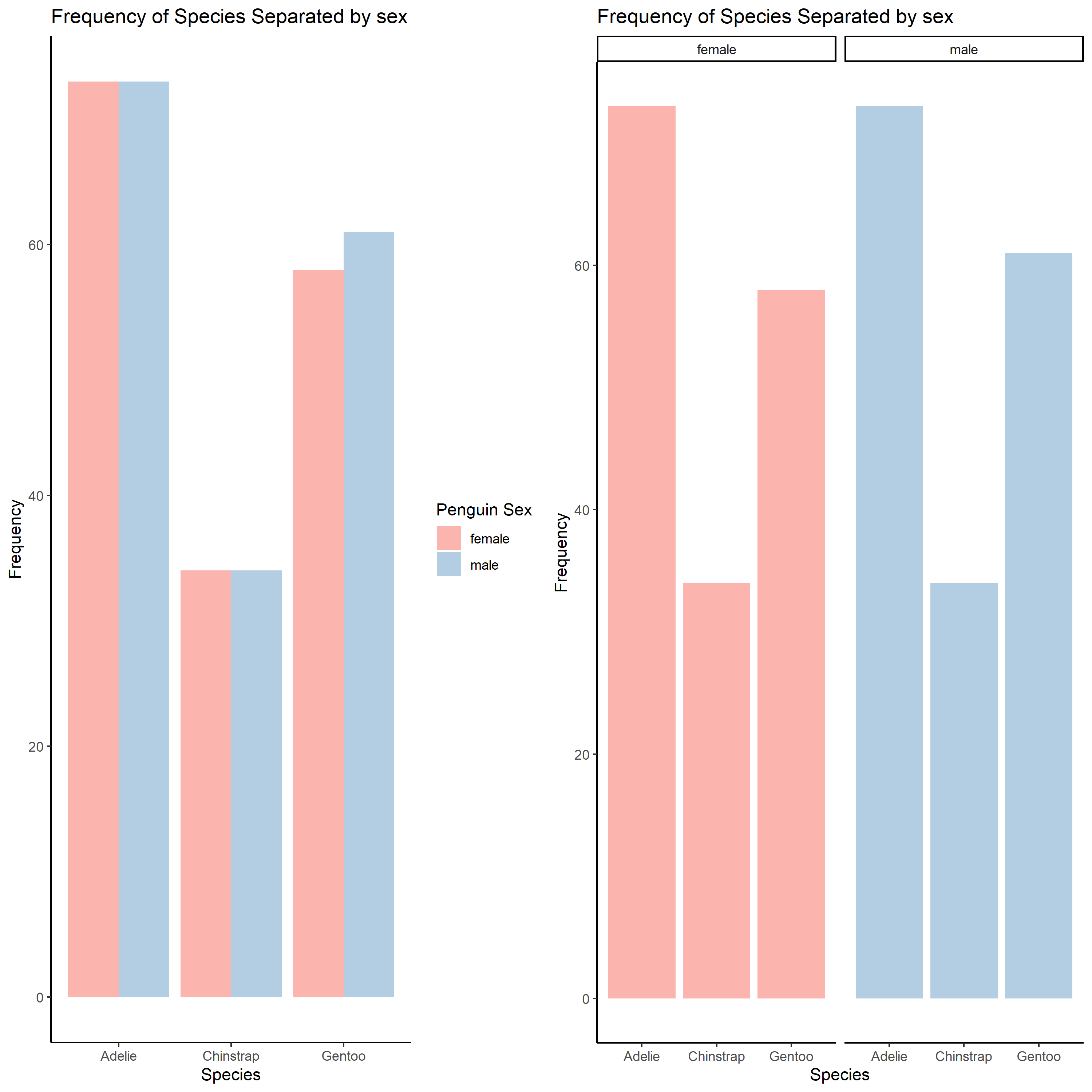
As you can see, both these graphs effectively display information. But depending on the method you use different relationships are highlighted with varying effiacy.
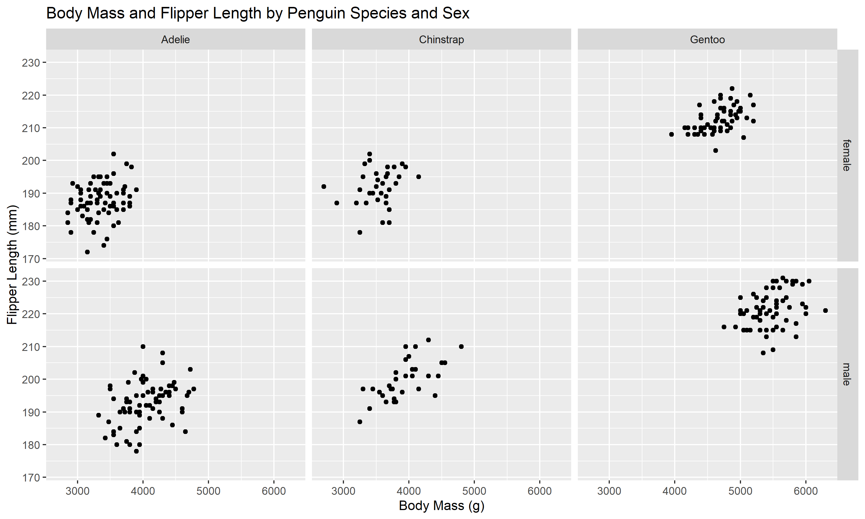
Finally, if you want to organize data by two categorical variables, you can use ggplot2::facet_grid() function. This function can be helpful to organize and customize the multi-panel figure.
grid <- ggplot(penguins, aes(x=body_mass_g, y=flipper_length_mm))+
  geom_point()+
  facet_grid(sex~species) + #create panels of sex and species
  labs(title="Body Mass and Flipper Length by Penguin Species and Sex", #change the title of the figure
       x="Body Mass (g)", #change the label of the x axis
       y="Flipper Length (mm)") #change the label of the y axis
grid #view the multi-panel figure
Summary
In this post, we went over the following methods for creating multi-panel plots.
- Using baseR par() parameter
- Using baseR layout() function
- Using patchwork package
- Using cowplot package
- Using ggpubr::ggarrange
In my opinion, the ggpubr::ggarrange method allows for the most flexibility for creating multi-panel figures and is the one that I would use if I was trying to create multi-panel figures. Additionally, we went over multi-panel plots with unique variable combinations:
- Marginal plots using layout() function
- Marginal plots using ggExtra::ggMarginal function
- Using ggplot2::facet_wrap to create panels differentiated by one discrete variable
- Using ggplot2::facet_grid to create panels differentiated by two discrete variables
Try one or more of these multi-panel methods with your data! Let me know here if this tutorial was helpful or not. What kinds of content would you like to see more on this blog?