Moving Pictures?! Animated Figures in R

Last updated on Tue, Dec 8, 2020 4 min read

Static plots can be difficult to process as a viewer and difficult to explain as a presenter. One technique to work with busy plots may be to embed transitions into them to help walk through them during oral presentations. We’ll walk through some gganimate transitions that may be helpful for walking through figures.

Load in dataset + relevant libraries

In all these examples, we will use the penguins dataset in the palmerpenguins package. Instructions to download this package can be found here. This package includes two datasets but we will use penguins. Before using this data in figures, we omitted any rows with one or more cells using the na.omit() function. Additionally, we will be loading in the following packages: ggplot2, RcolorBrewer, and gganimate.

library(palmerpenguins)

?penguins #can be used to find more information about the penguins dataset

data("penguins")
head(penguins)
penguins <- na.omit(penguins)  #remove any rows with missing values

library(ggplot2) # to create data visualizations 
library(RcolorBrewer) # for multiple color palettes
library(gganimate) # to add animations to visualizations

Continuous variable?

The transition_reveal() function reveals each new frame of a dimension gradually. Usually, this dimension is a continuous variable or a time series. The transition_time() function can be used for continuous variables or where the variables are representing specific points in time. In both of these functions, you can specify the range of the variable using the “range=" argument of these functions.

transition_time

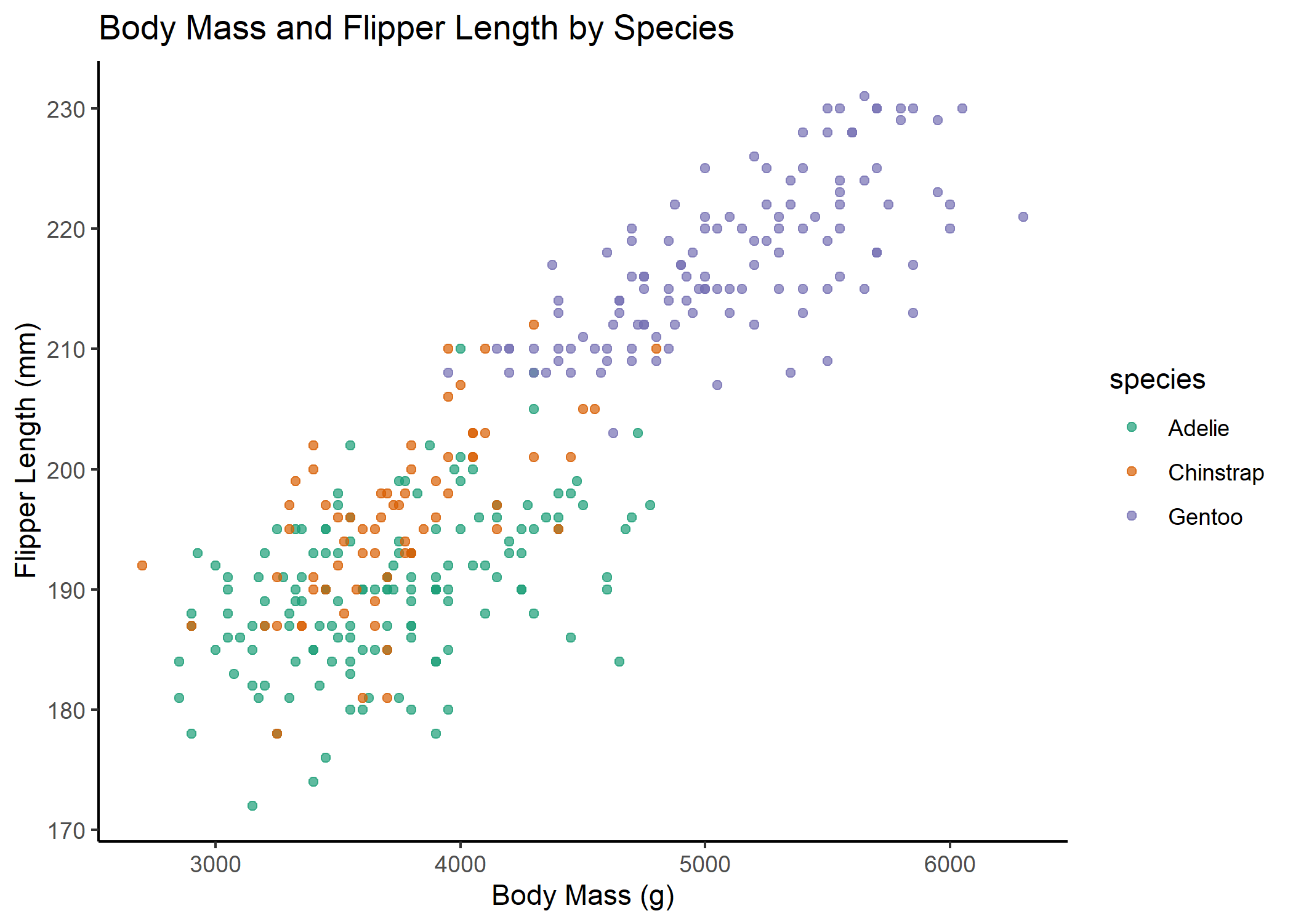
Static plot of body mass and flipper length by species:

bubstatic <- ggplot(penguins, aes(body_mass_g, flipper_length_mm, 
                                colour = species)) +
  geom_point(alpha=0.7, show.legend = T) + # alpha = opacity of points 
  scale_color_brewer(palette="Dark2")+ 
  theme_classic()+
  labs(x="Body Mass (g)", y="Flipper Length (mm)", # label axes
       title="Body Mass and Flipper Length by Species and Bill Length") # label figure
bubstatic # view static plot

Animated Plot:

bubanim <- ggplot(penguins, aes(body_mass_g, flipper_length_mm, 
                     colour = species)) +
  geom_point(alpha = 0.7, show.legend = F) +
  scale_color_brewer(palette="Dark2")+
  theme_classic()+
  labs(title = 'Year: {frame_time}', # label each frame of the animation 
       x = 'Body Mass (g)', y = 'Flipper Length (mm)') + # label axes
  transition_time(year) + # gganimate part; continuous time variable 
  ease_aes('linear') # adjusts the speed of the asethetic; smooths the animation out 
bubanim # view animated plot

With the animation, you can now discuss the relationship between body mass and flipper length across time.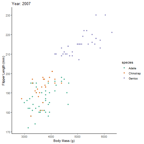

transition_reveal

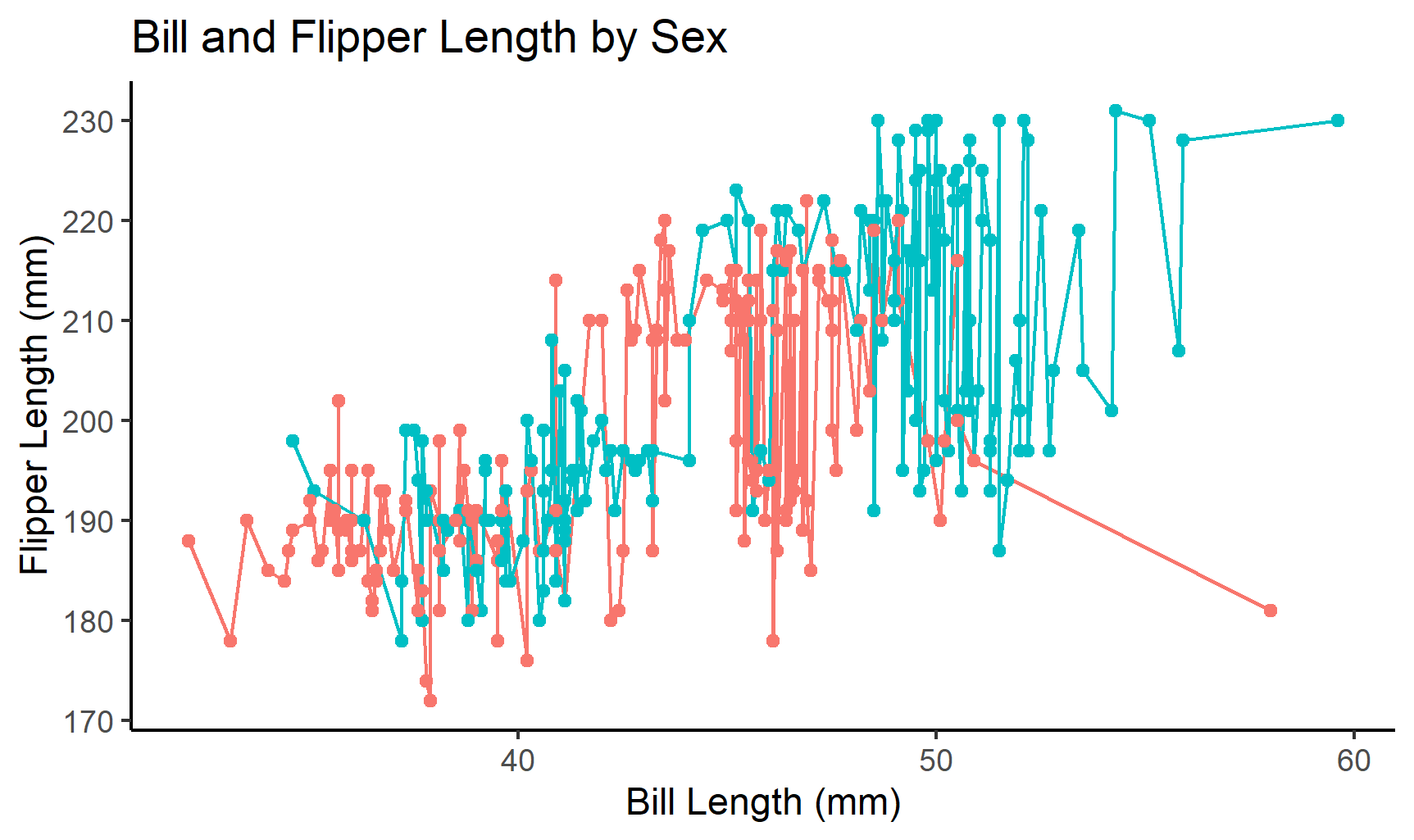
Static plot of bill and flipper length separated by sex:

linestatic <- ggplot(penguins, aes(x=bill_length_mm, y=flipper_length_mm, color=sex))+
  geom_line(show.legend=F)+
  geom_point(show.legend=F)+ 
  theme_classic()+
  labs(x="Bill Length (mm)", y= "Flipper Length (mm)", # label axes
       title="Bill and Flipper Length by Sex") # label figure
linestatic # view graph

Animated plot:

lineanim <- ggplot(penguins, aes(x=bill_length_mm, y=flipper_length_mm, color=sex))+
  geom_line(show.legend=F)+
  theme_classic()+
  labs(x="Bill Length (mm)", y= "Flipper Length (mm)", # label axes
       title="Bill and Flipper Length by Sex")+ # label figure 
  transition_reveal(bill_length_mm) #gganimate part; continuous variable 
lineanim # view animated graph

See how much more more sense it makes when you animate the plot! You can actually talk through the differences across sexes more clearly using this animation.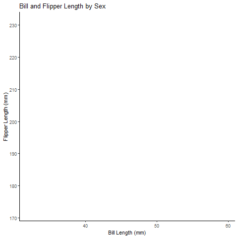

Discrete variable?

The transition_states() function animates the states of a discrete variable.

transition_states

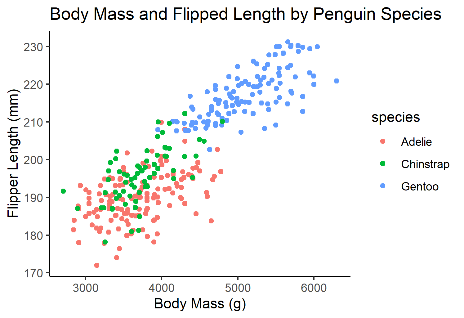
Static Plot of body mass and flipper length by species:

pointstatic <- ggplot(penguins, 
                  aes(x=body_mass_g, 
                      y= flipper_length_mm))+
  geom_point(aes(color=species),
             position="jitter", show.legend = T)+
  theme_classic()+
  labs(x="Body Mass (g)", y="Flipper Length (mm)",
       title="Body Mass and Flipped Length by Penguin Species")
pointstatic # view static plot

Animated Plot:

pointanim <- ggplot(penguins, 
          aes(x=body_mass_g, 
              y= flipper_length_mm))+
  geom_point(aes(color=species, group=1L), # choose the discrete variable aesthetic; the group= argument fades each group value into each other
             position="jitter", show.legend = F)+ 
  theme_classic()+
  labs(x="Body Mass (g)", y="Flipper Length (mm)", # label axes
       title="Body Mass and Flipped Length by Penguin Species")+
  #gganimate part     
  transition_states(species, # discrete variable
                    transition_length = 2, # length of transition between discrete variable groups
                    state_length = 1)+ # duration of animation on each group of the discrete variable
  ggtitle('Now showing {closest_state}',
          subtitle = 'Frame {frame} of {nframes}') # label each frame of the animation 
pointanim # view anim plot

See, with the animation its much easier to talk about the the relationship of body mass of each species individually and all the penguins together.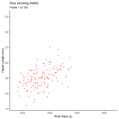

Summary

In this post, we went over the following methods for creating animations using continuous variables:

Using transition_time() function
Using transition_reveal() function

And animations using discrete variables:

Using transition_states() function

Try one or more of these transitions with your data! Let me know here if this tutorial was helpful or not. What kinds of content would you like to see more on this blog?